How to Build Decision Tree for Classification – (Step by Step Using Entropy and Gain)

In this Lesson, I would teach you how to build a decision tree step by step in very easy way, with clear explanations and diagrams.

Content

1. What are Decision Trees
2. Exercise for this Lesson
3. The ID3 Algorithm for Building Decision Trees
4. Step by Step Procedure
   • Step 1: Determine the Root of the Tree
   • Step 2: Calculate Entropy for The Classes
   • Step 3: Calculate Entropy After Split for Each Attribute
   • Step 4: Calculate Information Gain for each split 
   • Step 5: Perform the Split
   • Step 6: Perform Further Splits
   • Step 7: Complete the Decision Tree
5. Final Notes

1. What are Decision Trees

A decision tree is a tree-like structure that is used as a model for classifying data. A decision tree decomposes the data into sub-trees made of other sub-trees and/or leaf nodes.
A decision tree is made up of three types of nodes

• Decision Nodes: These type of node have two or more branches
• Leaf Nodes: The lowest nodes which represents decision
• Root Node: This is also a decision node but at the topmost level

The question is : How to we build a decision tree? Let’s see!

2. Exercise for this Lesson

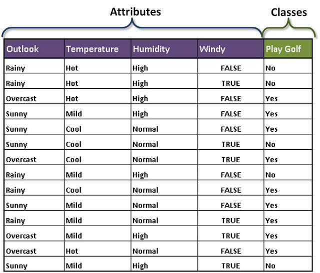
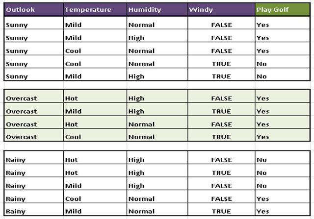
Consider the table below. It represent factors that affect whether John would go out to play golf or not. Using the data in the table, build a a decision tree to model that can be used to predict if John would play golf or not.

 

3. Algorithm for Building Decision Trees – The ID3 Algorithm(you can skip this!)

This is the algorithm you need to learn, that is applied in creating a decision tree. Although you don’t need to memorize it but just know it. It is called the ID3 algorithm by J. R. Quinlan. The algorithm uses Entropy and Informaiton Gain to build the tree.
Let:

S = Learning Set
A = Attibute Set
V = Attribute Values

Begin
Load learning sets  and create decision tree root node(rootNode), add learning set S into root not as its subset
For rootNode, compute Entropy(rootNode.subset) first
If Entropy(rootNode.subset) == 0 (subset is homogenious)
      return a leaf node

If Entropy(rootNode.subset)!= 0 (subset is not homogenious)
     compute Information Gain for each attribute left (not been used for spliting)
     Find attibute A with Maximum(Gain(S, A))
     Create child nodes for this root node and add to rootNode in the decision tree

For each child of the rootNode
   Apply ID3(S, A, V)
   Continue until a node with Entropy of 0 or a leaf node is reached
End

(You actually don’t have to worry trying to understand every bit of this algorithm. The application would make is very clear)

4. Step by Step Procedure for Building a Decision Tree

Here I would give you a simple step by step procedure that is super-easy to follow in creating a decision tree no matter how complex it could be.
Start by determining the root of the tree and the class column

Step 1: Determine the Decision Column

Since decision trees are used for clasification, you need to determine the classes which are the basis for the decision.
In this case, it it the last column, that is Play Golf column with classes Yes and No.

To determine the rootNode we need to compute the entropy.
To do this, we create a frequency table for the classes (the Yes/No column).

 

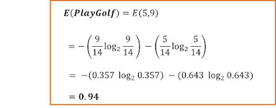
Step 2: Calculating Entropy for the classes (Play Golf)

In this step, you need to calculate the entropy for the Play Golf column and the calculation step is given below.

Step 3: Calculate Entropy for Other Attributes After Split

For the other four attributes, we need to calculate the entropy after each of the split.

• E(PlayGolf, Outloook)
• E(PlayGolf, Temperature)
• E(PlayGolf, Humidity)
• E(PlayGolf,Windy)

The entropy for two variables  is calculated using the formula.
(don’t worry if about this formula, its really easy doing the calculation ☺

There to calculate E(PlayGolf, Outlook), we would use the formula below:

Which is

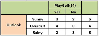
This formula may look unfriendly, but it is quite clear. The easiest way to approach this calculation is to create a frequency table for the two variables, that is PlayGolf and Outlook.

This frequency table is given below:

 

Using this table, we can then calculate E(PlayGolf, Outlook), which would then be given by the formula below

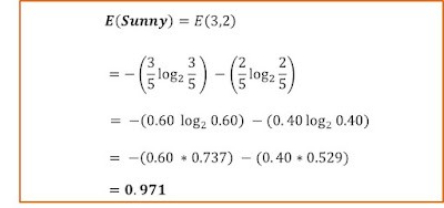
Let’s go ahead to calculate E(3,2)
We would not need to calculate the second and the third terms! This is because

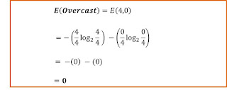
E(4, 0) = 0
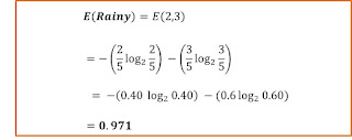
E(2,3) = E(3,2)
Isn’t this interesting!!!

Just for clarification, let’s show the the calculation steps
The calculation steps for E(4,0):

The calculation step for E(2,3) is given below

Time to put it all together.

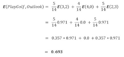
We go ahead to calculate the E(PlayGolf, Outlook) by substituting the values we calculated from E(Sunny), E(Overcast) and E(Rainy) in the equation:

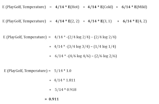
E(PlayGolf, Temperature) Calculation

Just like in the previous calculation, the calculation of E(PlayGolf, Temperature) is given below. It
It is easier to do if you form the frequency table for the split for Temperature as shown.

 

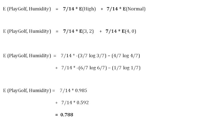
E(PlayGolf, Humidity) Calculation

Just like in the previous calculation, the calculation of E(PlayGolf, Humidity) is given below. It
It is easier to do if you form the frequency table for the split for Humidity as shown.

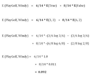
E(PlayGolf, Windy) Calculation

Just like in the previous calculation, the calculation of E(PlayGolf, Windy) is given below. It
It is easier to do if you form the frequency table for the split for Windy as shown.

 

Wow! That is so much work! So take break, walk around a little and take a glass of cold water.
Then we continue.
So now that we have all the entropies for all the four attributes, let’s go ahead to summarize them as shown in below:

1. E(PlayGolf, Outloook) = 0.693
2. E(PlayGolf, Temperature) = 0.911
3. E(PlayGolf, Humidity) = 0.788
4. E(PlayGolf,Windy) = 0.892

Step 4: Calculating Information Gain for Each Split

The next step is to calculate the information gain for each of the attributes. The information gain is calculated from the split using each of the attributes. Then the attribute with the largest information gain is used for the split.

The information gain is calculated using the formula:

Gain(S,T) = Entropy(S) – Entropy(S,T)

For example, the information gain after spliting using the Outlook attibute is given by:

Gain(PlayGolf, Outlook) = Entropy(PlayGolf) – Entropy(PlayGolf, Outlook)

So let’s go ahead to do the calculation

Gain(PlayGolf, Outlook) = Entropy(PlayGolf) – Entropy(PlayGolf, Outlook)
= 0.94 – 0.693 = 0.247


Gain(PlayGolf, Temperature) = Entropy(PlayGolf) – Entropy(PlayGolf, Temparature)
= 0.94 – 0.911 = 0.029

Gain(PlayGolf, Humidity) = Entropy(PlayGolf) – Entropy(PlayGolf, Humidity)
= 0.94 – 0.788 = 0.152

Gain(PlayGolf, Windy) = Entropy(PlayGolf) – Entropy(PlayGolf, Windy)
= 0.94 – 0.892 = 0.048

Having calculated all the information gain, we now choose the attribute that gives the highest information gain after the split.

Step 5: Perform the First Split

Draw the First Split of the Decision Tree
Now that we have all the information gain, we then split the tree based on the attribute with the highest information gain.

From our calculation, the highest information gain comes from Outlook. Therefore the split will look like this:

Now that we have the first stage of the decison tree, we see that we have one leaf node. But we still need to split the tree further.

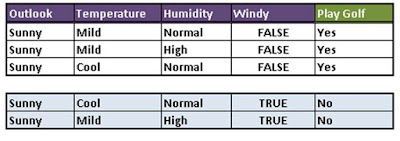
To do that, we need to also split the original table to create sub tables.
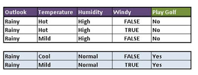
This sub tables are given in below.

From Table 3, we could see that the Overcast outlook requires no further split because it is just one homogeneous group. So we have a leaf node.

Step 6: Perform Further Splits

The Sunny and the Rainy attributes needs to be split

The Rainy  outlook can be split using either Temperature, Humidity or Windy.

Quiz 1: What attribute would best be used for this split? Why?

Answer:  Humidity. Because it produces homogenous  groups.

 

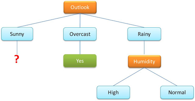
The Rainy attribute could be split using  High and Normal attributes and that would give us the tree below.

 

Figure 3: Split using the Humidity Attribute

Let’t now go ahead to do the same thing for the Sunny outlook
The Rainy  outlook can be split using either Temperature, Humidity or Windy.

Quiz 2: What attribute would best be used for this split? Why?
Answer:  Windy . Because it produces homogeneous  groups.

 

If we do the split using the Windy attribute, we would have the final tree that would require no further splitting! This is shown in Figure 4

Step 7: Complete the Decision Tree

The complete table is shown in Figure 4
Note that the same calculation that was used initially could also be used for the further splits. But that would not be necessary since you could just look at the sub table and be able to determine which attribute to use for the split.

Quiz: What does each of he color represent in the tree? 
Leave your answer in the comment box below

Figure 4: Final Decision Tree

 

5. Final Notes

Now we have successfully completed the decision tree.
I think we need to celebrate with a bottle of beer!
This is how easy it is to build a decision three. Remember, the initial steps of calculating the entropy and the gain is the most difficult part. But after that, everything falls into place.

Do let me know if you have any challenges. Write me in the comment box below or in the form at the left of this page.


Thanks for reading!!