Conditional Probability – Introduction to Bayes’ Rule

Bayes Rule is based on Conditional Probability which we have been discussing in the previous 3 lessons.

• Conditional Probability – Basics
• Conditional Probability – Multiplication Law
• Conditional Probability – Law of Total Probability

So I recommend you start from the basics. This  is because you need these basics to understand Bayes’ Rule.

Now, we would state Bayes’ rule and you will see it’s the same as what we already derived.

Let A and B1, . . . , Bn be events such that Bi are disjoint,

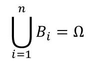
and P(Bi) > 0 for all i, then:

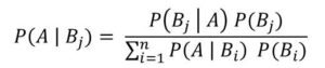
Let’s take some examples to illustrate how it works.

Example 1

Bayes’ rule was applied in diagnosing coronary artery disease. This is through a procedure called cardiac fluoroscopy. This procedure determines if there is calcification of the coronary arteries and hence diagnose coronary artery disease.

From the test carried out, number of arteries calcified could be determined. If it is 0, 1, 2 or 3.

Let T0, T1, T2, T3 denote these events.

Also let D+ denote that the disease is present

And D- denotes that the disease is absent

The results of the studies is presented in the table below

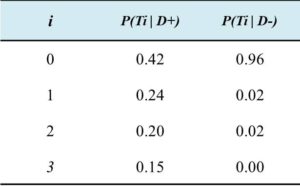
Now we need to calculate:

1. chances that the patient have the disease given that no artery is calcified – P(D+ | T0)

Let’s assume that the P(D+) is 0.05

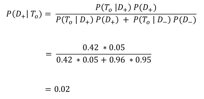
Applying Bayes’ rule to the above table, we have:

Now, we have P(D+) = 0.5

Therefore P(D-) = 1 – P(D+) = 0.95

So :

Exercises

1. Find  the chances that patient have the disease given that only on artery is calcified – P(D+ | T1)
2. Calculate the same values in Example 1, this time using P(D+) = 0.92

In the next lesson, we would further examine Bayes’ Rule using other examples.